Timber Flat Roof Beam Design [Structural Calculation]
When it comes to building a durable flat roof, proper timber beam design is crucial.
Not only does it ensure the structural integrity of your home or building, but it also adds to its aesthetic appeal.
However, the process of designing such a roof can be overwhelming, especially for those without a background in structural engineering.
That’s why we break down the basics of timber flat roof beam design.
In this post we’ll go through, step-by step, how to dimension and design the elements of the flat roof according to the timber Eurocode EN 1995-1-1:2004.
Not much more talk, let’s dive into it.
🙋♀️ What is a flat timber roof?
The flat timber roof is a structural roof system that – as the name says – has no inclination or just a very small for water drainage purposes. The vertical loads are usually carried by secondary beams and transferred to primary beams, which are supported by columns. Wind bracing straps or timber boards are used for the horizontal wind bracing system and to transfer the horizontal loads down to the foundation.
As already mentioned, there is different types of the flat roof, meaning that the different elements can be built with different materials and systems.
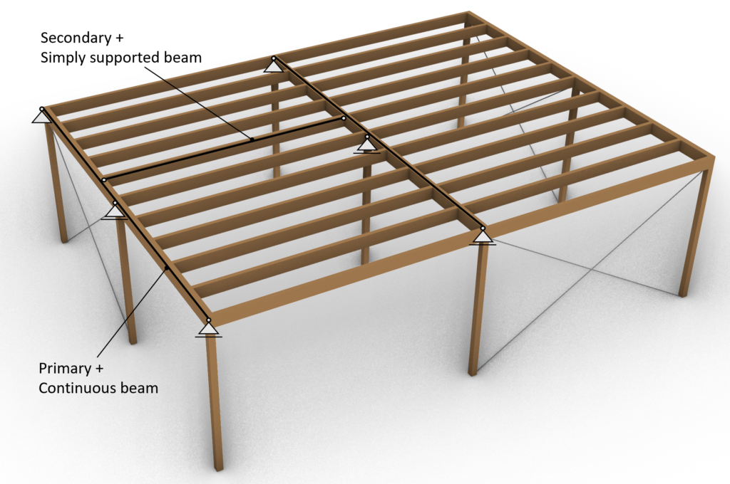
One example of the flat roof type can be seen in the next picture, where the secondary timber beams span between the primary beams.
Steel rods can be used for both the horizontal roof and vertical bracing system. The primary beams are supported by timber columns, which act as supports for the primary beams.
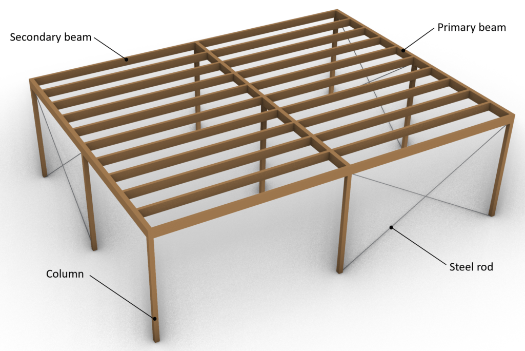
.. and because 3D models are even better than 2D pictures here is also the 3D model.
We haven’t covered wind bracing systems yet, – how they work, why we need them – but would you be interested in learning more? Let me know in the comments below.
👆 Static system of the flat roof beams
The static system of the flat roof is actually split up in 2 or more static systems, depending on whether we also look at the horizontal stiffening by plates or steel rods and if the columns should also be included in the flat roof calculation.
But we decided to look at the horizontal bracing in another article.
As we can see in the picture above, in our example, there are primary and secondary beams.
The loads (wind, snow, live, dead) are first carried by the secondary beams (modelled as beams – surprise😁) and then transferred to the primary beams, which means that the vertical support forces of the secondary beams are applied as pointloads on the primary beams.
Now let’s look at those static systems because words are not as explanatory as images.
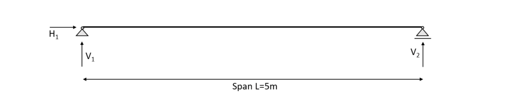
The static system of the secondary beam is a simply supported beam.
.. and the static system of the outer primary beam is a continous beam.
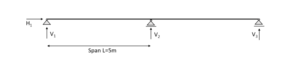
But how are both 2-dimensional static systems connected to each other now? This can be confusing.
Let’s look at a 3-dimensional picture of the roof.
If this is still a bit unclear – stick with us – it’s getting a lot clearer when we look at the load transfer.
As the flat roof has basically no or a very small inclination and as we will see later, all loads are applied perpendicular to the beams.
Therefore, the beams will only act in bending. Let’s find and apply the loads in the following section.
⬇️ Characteristic loads of the flat roof
The loads will not be derived in this article. We explained the calculation of dead, live, wind and snow loads for flat roofs thoroughly in previous articles.
In case the flat roof is part of a canopy structure, Eurocode includes an extra section which calculates the wind load specifically for canopy structures.
In this tutorial, we assume that the structure is closed (building) and wind can’t blow from underneath the roof.
The defined load values are estimations from the previous calculations.
| $g_{k}$ | 1.08 kN/m2 | Characteristic value of dead load |
| $q_{k}$ | 1.0 kN/m2 | Characteristic value of live load |
| $s_{k}$ | 0.8 kN/m2 | Characteristic value of snow load |
In this calculation, we will only focus on the external wind pressure for areas of 10 m2.
Wind direction front and side
| $w_{k.F}$ | -0.7 kN/m2 | Characteristic value of wind load Area F |
| $w_{k.G}$ | -0.47 kN/m2 | Characteristic value of wind load Area G |
| $w_{k.H}$ | -0.27 kN/m2 | Characteristic value of wind load Area H |
| $w_{k.I}$ | -(+)0.08 kN/m2 | Characteristic value of wind load Area I |
Check out this article to see how you define the wind load areas F, G, H and I.
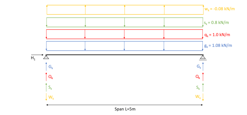
The following picture presents the static system of the secondary beam with its line loads applied. The section that is presented in Figure: 2D static systems with 3D context is used for this example.
Due to simplicity, this tutorial looks only at the wind load from the front. Therefore, the wind load $w_{k.I} = -(+)0.08kN/m^2$ is applied to the beam and because the wind load on roofs is usually suction we will only use the value of $-0.08kN/m^2$.
But we only do that so the calculation and this tutorial are more clean and easier to follow. In “reality” you should consider all values.
As the value of is almost 0 the contribution of the wind load in that area is also almost 0.
| $g_{k}$ | 1.08 kN/m2 * 1.0m = 1.08 kN/m |
| $q_{k}$ | 1.0 kN/m2 * 1.0m = 1.0 kN/m |
| $s_{k}$ | 0.8 kN/m2 * 1.0m = 0.8 kN/m |
| $w_{k}$ | -0.08 kN/m2 * 1.0m = -0.08 kN/m |
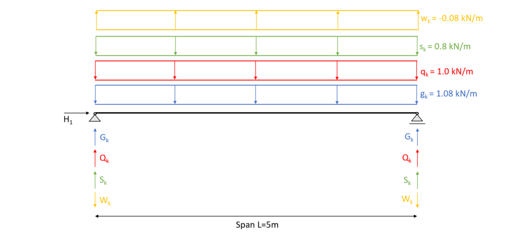
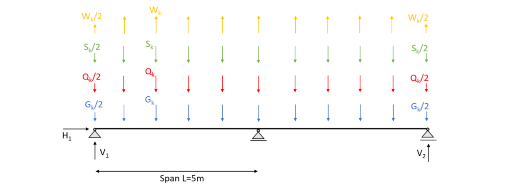
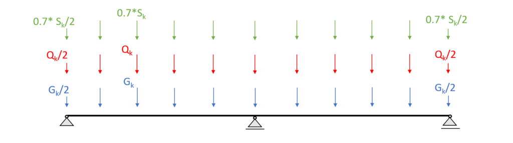
As we can see, the characteristic actions (loads) applied on the secondary beam lead to reaction forces ($W_{k}, S_{k}, Q_{k}, G_{k}$) of the simply supported beam.
Those reaction forces now become the characteristic forces (Point loads) on the continuous beam (primary beam).
Also remember❗
In reality, the wind point loads don’t have the same value because of the different wind areas discussed above, but also more in detail here.
➕ Load combinations of the flat roof
Luckily we have already written an extensive article about what load combinations are and how we use them. In case you need to brush up on it you can read the blog post here.
We choose to include $w_{k.I.}$ = -0.08 kN/m2 as the wind load in the load combinations, as this is the wind load that is applied to the section we look at, and to keep the calculation clean.
In principle, you should consider all load cases. However, with a bit more experience, you might be able to exclude some of the values.
In modern FE programs, multiple values for the wind load can be applied and load combinations automatically generated. So the computer is helping us a lot.
Just keep in mind that you should include all wind loads, but because of simplicity we do only consider 1 value in this article😁.
ULS Load combinations
| LC1 | $1.35 * 1.08 \frac{kN}{m} $ |
| LC2 | $1.35 * 1.08 \frac{kN}{m} + 1.5 * 1.0 \frac{kN}{m}$ |
| LC3 | $1.35 * 1.08 \frac{kN}{m} + 1.5 * 1.0 \frac{kN}{m} + 0.7 * 1.5 * 0.8 \frac{kN}{m}$ |
| LC4 | $1.35 * 1.08 \frac{kN}{m} + 0 * 1.5 * 1.0 \frac{kN}{m} + 1.5 * 0.8 \frac{kN}{m}$ |
| LC5 | $1.35 * 1.08 \frac{kN}{m} + 1.5 * 1.0 \frac{kN}{m} + 0.7 * 1.5 * 0.8 \frac{kN}{m} + 0.6 * 1.5 * (-0.08 \frac{kN}{m}) $ |
| LC6 | $1.35 * 1.08 \frac{kN}{m} + 0 * 1.5 * 1.0 \frac{kN}{m} + 1.5 * 0.8 \frac{kN}{m} + 0.6 * 1.5 * (-0.08 \frac{kN}{m}) $ |
| LC7 | $1.35 * 1.08 \frac{kN}{m} + 0 * 1.5 * 1.0 \frac{kN}{m} + 0.7 * 1.5 * 0.8 \frac{kN}{m} + 1.5 * (-0.08 \frac{kN}{m}) $ |
| LC8 | $1.35 * 1.08 \frac{kN}{m} + 1.5 * 0.8 \frac{kN}{m} $ |
| LC9 | $1.35 * 1.08 \frac{kN}{m} + 1.5 * (-0.08 \frac{kN}{m}) $ |
| LC10 | $1.35 * 1.08 \frac{kN}{m} + 1.5 * 1.0 \frac{kN}{m} + 0.6 * 1.5 * (-0.08 \frac{kN}{m}) $ |
| LC11 | $1.35 * 1.08 \frac{kN}{m} + 1.5 * (-0.08 \frac{kN}{m}) + 0.7 * 1.5 * 0.8 \frac{kN}{m} $ |
| LC12 | $1.35 * 1.08 \frac{kN}{m} + 1.5 * 2.12 \frac{kN}{m} + 0.6 * 1.5 * (-0.08 \frac{kN}{m})$ |
Characteristic SLS Load combinations
| LC1 | $1.08 \frac{kN}{m} $ |
| LC2 | $1.08 \frac{kN}{m} + 1.0 \frac{kN}{m}$ |
| LC3 | $1.08 \frac{kN}{m} + 1.0 \frac{kN}{m} + 0.7 * 0.8 \frac{kN}{m}$ |
| LC4 | $1.08 \frac{kN}{m} + 1.0 \frac{kN}{m} + 0.6 * (-0.08 \frac{kN}{m})$ |
| LC5 | $1.08 \frac{kN}{m} + 1.0 \frac{kN}{m} + 0.7 * 0.8 \frac{kN}{m} + 0.6 * (-0.08 \frac{kN}{m}) $ |
| LC6 | $1.08 \frac{kN}{m} + 0 * 1.0 \frac{kN}{m} + 0.8 \frac{kN}{m} + 0.6 * (-0.08 \frac{kN}{m}) $ |
| LC7 | $1.08 \frac{kN}{m} + 0 * 1.0 \frac{kN}{m} + 0.7 * 0.8 \frac{kN}{m} + (-0.08 \frac{kN}{m}) $ |
| LC8 | $1.08 \frac{kN}{m} + 0.8 \frac{kN}{m}$ |
| LC9 | $1.08 \frac{kN}{m} + (-0.08 \frac{kN}{m}) $ |
| LC10 | $1.08 \frac{kN}{m} + 1.0 \frac{kN}{m} + 0.6 * (-0.08 \frac{kN}{m}) $ |
| LC11 | $1.08 \frac{kN}{m} + (-0.08 \frac{kN}{m}) + 0.7 * 0.8 \frac{kN}{m} $ |
| LC12 | $1.08 \frac{kN}{m} + 0 * 1.0 \frac{kN}{m} + 0.8 \frac{kN}{m}$ |
| LC13 | $1.08 \frac{kN}{m} + 0 * 1.0 \frac{kN}{m} + (-0.08 \frac{kN}{m})$ |
👉 Definition timber material properties
🪵 Timber beam material
For this blog post/tutorial we are choosing a Structural timber C24. More comments on which timber material to pick and where to get the properties from were made here.
The following characteristic strength and stiffness parameters were found online from a manufacturer.
| Bending strength $f_{m.k}$ | 24 $\frac{N}{mm^2}$ |
| Tension strength parallel to grain $f_{t.0.k}$ | 14 $\frac{N}{mm^2}$ |
| Tension strength perpendicular to grain $f_{t.90.k}$ | 0.4 $\frac{N}{mm^2}$ |
| Compression strength parallel to grain $f_{c.0.k}$ | 21 $\frac{N}{mm^2}$ |
| Compression strength perpendicular to grain $f_{c.90.k}$ | 2.5 $\frac{N}{mm^2}$ |
| Shear strength $f_{v.k}$ | 4.0 $\frac{N}{mm^2}$ |
| E-modulus $E_{0.mean}$ | 11.0 $\frac{kN}{mm^2}$ |
| E-modulus $E_{0.g.05}$ | 9.4 $\frac{kN}{mm^2}$ |
⌚ Modification factor $k_{mod}$
If you do not know what the modification factor $k_{mod}$ is, we wrote an explanation to it in a previous article, which you can check out.
Since we want to keep everything as short as possible, we are not going to repeat it in this article – we are only defining the values of $k_{mod}$.
For a residential house which is classified as Service class 1 according to EN 1995-1-1 2.3.1.3 we extract the following load durations for the different loads.
| Self-weight/dead load | Permanent |
| Live load, Snow load | Medium-term |
| Wind load | Instantaneous |
From EN 1995-1-1 Table 3.1 we get the $k_{mod}$ values for the load durations and a structural wood C24 (Solid timber).
| $k_{mod}$ | |||
|---|---|---|---|
| Self-weight/dead load | Permanent action | Service class 1 | 0.6 |
| Live load, Snow load | Medium term action | Service class 1 | 0.8 |
| Wind load | Instantaneous action | Service class 1 | 1.1 |
🦺 Partial factor for material properties $\gamma_{M}$
According to EN 1995-1-1 Table 2.3 the partial factor $\gamma_{M}$ is defined as
$\gamma_{M} = 1.3$
📏 Assumption of width and height of beams
We are defining the width w and height h of the C24 structural wood secondary beam Cross-section as
Width w = 120 mm
Height h = 240 mm
.. and the primary beam as
Width w = 160 mm
Height h = 280 mm
💡 We highly recommend doing any calculation in a program where you can always update values and not by hand on a piece of paper!
I made that mistake in my bachelor. In any course and even in my bachelor thesis, I calculated everything except the forces (FE program) on a piece of paper.
Now that we know the width and the height of the beam Cross-section we can calculate the Moment of inertias $I_{y}$ and $I_{z}$ of the secondary beam.
$I_{y} = \frac{w \cdot h^3}{12} = \frac{120mm \cdot (240mm)^3}{12} = 1.382 \cdot 10^8 mm^4 $
$I_{z} = \frac{w^3 \cdot h}{12} = \frac{(120mm)^3 \cdot 240mm}{12} = 3.456 \cdot 10^7 mm^4 $
.. and the primary beam
$I_{y} = \frac{w \cdot h^3}{12} = \frac{160mm \cdot (280mm)^3}{12} = 2.927 \cdot 10^8 mm^4 $
$I_{z} = \frac{w^3 \cdot h}{12} = \frac{(160mm)^3 \cdot 280mm}{12} = 9.557 \cdot 10^7 mm^4 $
🆗 ULS Design – secondary beam
In the ULS (ultimate limit state) Design we verify the stresses in the timber members due to bending, shear, normal forces and buckling.
However, since all the loads are perpendicular to the beams, there is no axial force in the beams and therefore no buckling.
In order to calculate the stresses of the beams, we need to calculate the Bending Moments and Shear forces due to different loads.
🧮 Calculation of bending moment and shear forces
Before we start calculating anything we need to pick out the worst case loadcombination. In our case that is load combination 3 which we apply to the simply supported beam.
Load combination 3
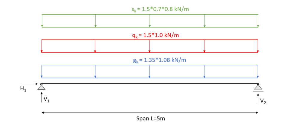
Adding up those line loads leads to a design line load of
$p_{d} = 1.35 * 1.08 \frac{kN}{m} + 1.5 * 1.0 \frac{kN}{m} + 1.5 * 0.7 * 0.8 \frac{kN}{m} = 3.8 \frac{kN}{m}$
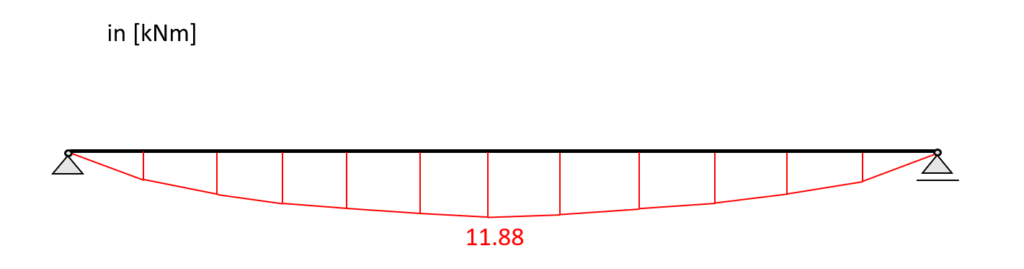
Load combination 3 – Bending moments
The highest bending moment in a simply supported beam is found in the midspan and can be calculated with the following formula:
$M_{d} = p_{d} \cdot \frac{l^2}{8}$
Where
- l = 5m is the length of span
Applying that to our situation leads to a bending moment of
$M_{d} = 3.8 \frac{kN}{m} \cdot \frac{(5m)^2}{8} = 11.875 kNm$
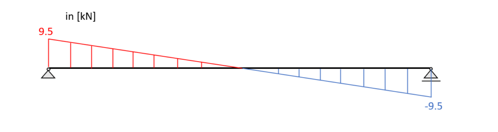
Load combination 3 – Shear forces
Like for bending Load combination 3 leads to the most critical shear force. The highest shear force in a simply supported beam is found near the 2 supports and can be calculated with the following formula:
$V_{d} = p_{d} \cdot \frac{l}{2}$
putting in the values in the formula leads to a max. shear force of
$V_{d} = 3.8 \frac{kN}{m} \cdot \frac{5m}{2} = 9.5 kN$
🔎 Bending Verification
From the max. bending moment in the span (11.88 kNm) we can calculate the stress in the most critical cross section as
Bending stress:
$\sigma_{m} = \frac{M_{d}}{I_{y}} \cdot \frac{h}{2} = \frac{11.88 kNm}{1.382 \cdot 10^{-4}m^4} \cdot \frac{0.24m}{2} = 10.31 MPa$
Resistance stresses of the timber material:
$ f_{d} = k_{mod} \cdot \frac{f_{k}}{\gamma_{m}} $
| LC3 (M-action) | $k_{mod.M} \cdot \frac{f_{m.k}}{\gamma_{m}} $ | $0.8 \cdot \frac{24 MPa}{1.3} $ | $14.77 MPa $ |
Utilization according to EN 1995-1-1 (6.11)
$\eta = \frac{\sigma_{m}}{f_{m.d}} = 0.70 < 1.0$
👨🏫 Shear Verification
From the max. shear force (midsupport: 9.5 kN) we can calculate the shear stress in the most critical cross section.
Shear stress:
$\tau_{d} = \frac{3V}{2 \cdot w \cdot h} = \frac{3 \cdot 9.5 kN}{2 \cdot 0.12m \cdot 0.24m} = 0.495 MPa$
Resistance stresses of the timber material:
$ f_{v} = k_{mod.M} \cdot \frac{f_{v}}{\gamma_{m}} $
$ f_{v} = 0.8 \cdot \frac{4 MPa}{1.3} = 2.46 MPa$
Utilization according to EN 1995-1-1 (6.13)
$\eta = \frac{\tau_{v}}{f_{v}} = 0.2 < 1.0$
👩🏫 SLS Design – Secondary beam
We also discussed the SLS design a bit more in detail in a previous article. In this blog post we are not explaining too much but rather show the calculations and its results😊
🖋️ Instantaneous deformation $u_{inst}$
$u_{inst}$ (instantaneous deformation) of our beam can be calculated with the load of the characteristic SLS load combination.
As for the bending moments and shear forces, load combination 3 is the most critical one. Load combination 3 in SLS applies the following loads to the simply supported beam.
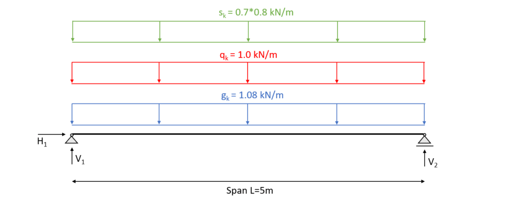
Adding up those line loads leads to a characteristic SLS line load of
$p_{k} = 1.08 \frac{kN}{m} + 1.0 \frac{kN}{m} + 0.7 * 0.8 \frac{kN}{m} = 2.64 \frac{kN}{m}$
The deflection of a simply supported beam is calculated with the following formula as
$u_{inst} = \frac{5}{384} \cdot p_{k} \cdot \frac{l^4}{E_{0.g.mean} \cdot I_{y}}$
Inserting the values of “our” beam leads to a instantaneous deformation of
$u_{inst} = \frac{5}{384} \cdot 2.64 \frac{kN}{m} \cdot \frac{(5m)^4}{1.1 \cdot 10^7 \frac{kN}{m^2} \cdot 1.382 \cdot 10^{-4} m^{4}} $
$u_{inst}$ = 14.13mm
Limit
EN 1995-1-1 Table 7.2 recommends values for $w_{inst}, w_{net.fin}$ and $w_{fin}$ which should not be exceeded for a simply supported beam.
| $w_{inst}$ | $w_{net.fin}$ | $w_{fin}$ |
| $L/300$ to $L/500$ | $L/250$ to $L/350 $ | $L/150$ to $L/300 $ |
With a beam length (span) of L=5m we get the following values.
| $w_{inst}$ | $w_{net.fin}$ | $w_{fin}$ |
| 16.67mm to 10mm | 20mm to 14.3mm | 33.3mm to 16.67mm |
Utilization
$\eta = \frac{u_{inst}}{w_{inst}} = \frac{14.13mm}{16.67mm} = 0.85 < 1$
🏇 Final deformation $u_{fin}$
$u_{fin}$ (final deformation) of our beam can be calculated by adding the creep deformation $u_{creep}$ to the instantaneous deflection $u_{inst}$.
Therefore, we will calculate the creep deformation. This tutorial is already very long, so we are not going to show all the steps, but instead save space and only write down the result.
But don’t worry, we have explained how to calculate the creep deformation in this article. Let me know in the comments below if you struggle with calculating the creep deformation.
The creep deformation of LC3 is calculated as
$u_{creep}$ = 3.98mm
Adding the creep to the instantaneous deflection leads to the final deflection.
$u_{fin} = u_{inst} + u_{creep} = 14.13mm + 3.98mm= 18.11mm$
Limit of $u_{fin}$ according to EN 1995-1-1 Table 7.2
$w_{fin}$ = l/150 = 5.0m/150 = 33.33 mm
Utilization
$\eta = \frac{u_{fin}}{w_{fin}} = \frac{18.11mm}{33.33mm} = 0.54$
Now that the secondary beam is verified, and the cross-sectional dimensions are found, we can go further and apply the support forces of the secondary beam onto the primary beam.
Let’s do that in the next section.
🆗 ULS Design – primary beam
First, let’s calculate the support forces of the secondary beam due to the different characteristic loads, so that we then can go ahead and apply them on the secondary beam.
The support forces are calculated as
$V = Line load * \frac{l}{2}$
| $G_{k}$ | 2.7 kN |
| $Q_{k}$ | 2.5 kN |
| $S_{k}$ | 2.0 kN |
| $W_{k}$ | -0.2 kN |
In order to calculate the stresses of the beams, we need to calculate the Bending Moments and Shear forces due to the different loads or the leading load combination to be more precise.
🧮 Calculation of bending moment and shear forces
As for the secondary beam Load combination 3 is also the most critical one for the primary beam.
Load combination 3
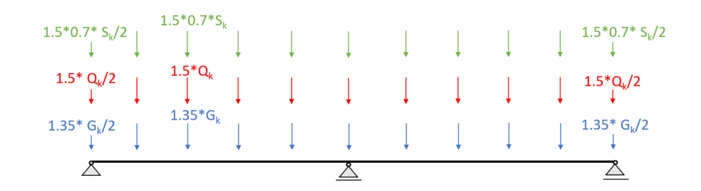
Now one can calculate the bending moments and forces either with an approximation of transforming the Point loads into a line load and finding the bending moment with tables for continuous beams – or by using a beam/FE program.
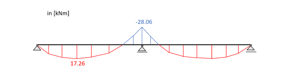
Load combination 3 – Bending moments
The highest bending moment in a continuous beam is found in the midsupport by a beam program as
$M_{d} = 28.08 kNm$
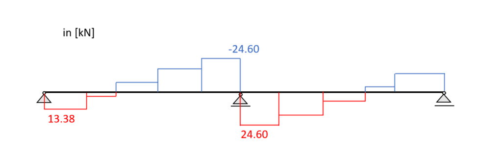
Load combination 3 – Shear forces
The highest shear force in a continuous beam is found in the midsupport by a beam program as
$V_{d} = 24.6 kN$
🔎 Bending Verification
From the max. bending moment at the midsupport (28.06 kNm) we can calculate the stress in the most critical cross section as
Bending stress:
$\sigma_{m} = \frac{M_{d}}{I_{y}} \cdot \frac{h}{2} = \frac{28.06 kNm}{2.927 \cdot 10^{-4} m^4} \cdot \frac{0.28m}{2} = 13.42 MPa$
| LC3 (M-action) | $k_{mod.M} \cdot \frac{f_{m.k}}{\gamma_{m}} $ | $0.8 \cdot \frac{24 MPa}{1.3} $ | $14.77 MPa $ |
Utilization according to EN 1995-1-1 (6.11)
$\eta = \frac{\sigma_{m}}{f_{m.d}} = 0.91 < 1.0$
👨🏫 Shear Verification
From the max. shear force (midsupport: 24.6 kN) we can calculate the shear stress in the most critical cross section.
Shear stress:
$\tau_{d} = \frac{3V}{2 \cdot w \cdot h} = \frac{3 \cdot 24.6 kN}{2 \cdot 0.16m \cdot 0.28m} = 0.824 MPa$
Resistance stresses of the timber material:
$ f_{v} = 0.8 \cdot \frac{4 MPa}{1.3} = 2.46 MPa$
Utilization according to EN 1995-1-1 (6.13)
$\eta = \frac{\tau_{v}}{f_{v}} = 0.34 < 1.0$
👩🏫 SLS Design – Primary beam
🖋️ Instantaneous deformation $u_{inst}$
As for the bending moments and shear forces Load combination 3 is the most critical one. Load combination 3 in SLS applies the following loads to the simply supported beam.
As for the forces we calculate the deflection with a beam program. The instantaneous deformation is found to be
$u_{inst} = 7.7mm$
Limit
EN 1995-1-1 Table 7.2 recommends values for $w_{inst}, w_{net.fin}$ and $w_{fin}$ which should not be exceeded for a simply supported beam.
Since we have a continuous beam, but the Standard only recommends values for simply supported beams, we also use those values for this tutorial.
| $w_{inst}$ | $w_{net.fin}$ | $w_{fin}$ |
| $L/300$ to $L/500$ | $L/250$ to $L/350 $ | $L/150$ to $L/300 $ |
With a beam length (span) of L=5m, we get the following values.
| $w_{inst}$ | $w_{net.fin}$ | $w_{fin}$ |
| 16.67mm to 10mm | 20mm to 14.3mm | 33.3mm to 16.67mm |
Utilization
$\eta = \frac{u_{inst}}{w_{inst}} = \frac{7.7mm}{16.67mm} = 0.46 < 1$
🏇 Final deformation $u_{fin}$
The creep deformation of LC3 is found to be
$u_{creep}$ = 2.16mm
Adding the creep to the instantaneous deflection leads to the final deflection.
$u_{fin} = u_{inst} + u_{creep} = 7.7mm + 2.16mm= 9.86mm$
Limit of $u_{fin}$ according to EN 1995-1-1 Table 7.2
$w_{fin}$ = l/150 = 5.0m/150 = 33.33 mm
Utilization
$\eta = \frac{u_{fin}}{w_{fin}} = \frac{9.86mm}{33.33mm} = 0.30$
🤝 Conclusion
Now that both primary and secondary beams are verified for bending, shear and deflection, we can finally say that the cross-section heights and widths are verified – check.✔️
The next element a structural engineer needs to dimension are the timber columns.
If you are interested in the design of other timber roofs, then check out our other guides:
But now I am curious to hear from you: Which is your favourite roof system? Which flat roof layout have you already used in a design?
Let me know in the comments✍️
❓ Howe Truss FAQ
The main purpose of a timber flat roof beam is to provide structural support for the roof. The beams transfer the weight of the roof and other loads such as wind, snow, and live load to the supporting walls or columns of the structure/building.
A Proper design of the beams ensures the structural safety of the flat roof and protects it from potential collapse.
![How To Dimension Rafters Of Purlin Roofs? [Structural Guide]](https://www.structuralbasics.com/wp-content/uploads/2022/03/How-to-design-rafters-of-purlin-roofs-768x439.jpg)